From the previous topic, we learned about test of significance, a procedure for comparing observed data with a claim or hypothesis or predicted data.
- This test of significant is used to test e claim about an unknown population and for testing the research hypothesis against the H0.
- Null hypothesis (H0) denotes that there is no difference between two population mean.
- In some statistical analysis this researchers need to compare the means of two or more variables or groups of data to easier their work .In case of two variables, comparison of mean can be measured by some specific significance test .
- Here we are going to know about such a hypothesis test called as student’s t-test.
- Comparison of means of two samples is occurred to find whether difference of two means of two groups is significant or not.
Student’s t-test
A t-test is a statistical test that is used to compare the means of two groups. It is often used in hypothesis testing to determine whether a process or treatment actually has an effect on the population of interest, or whether two groups are different from one another.
Best safe and secure cloud storage with password protection
Get Envato Elements, Prime Video, Hotstar and Netflix For Free
Best Money Earning Website 100$ Day
#1 Top ranking article submission website

Discovery of student’s t-test
- William Scaly Gusset discovered student’s t-test in 1908.
- Born – June 13,1908 (at Canterbury, Kent, England )
Died – October 16, 1927 (aged 61 at Beaconsfield, Buckinghamshire, England) - Known for student’s t-distribution.
- Test of significance of difference in means are discussed under two heads:
-
-
-
-
-
- t-test for large samples, (This test is also called Z-test)
- t-test for small samples.
-
-
-
-
- t-test for small samples are applied as
-
-
-
-
-
- Unpaired t-test (two independent samples) and
- Paired t-test (single sample correlated observations)
-
-
-
-
- Two essential conditions for these tests are
-
-
-
-
- It should be ensured that samples are selected randomly, and
- There should be homogeneity of variances in the two samples.
-
-
-
Formula of student’s t-test (and Z test)

A. Estimating the difference of means of two samples
-
-
- We already know, mean is an arithmetic average of a sample or population.
-

B. Estimating the Standard error of that difference
-
-
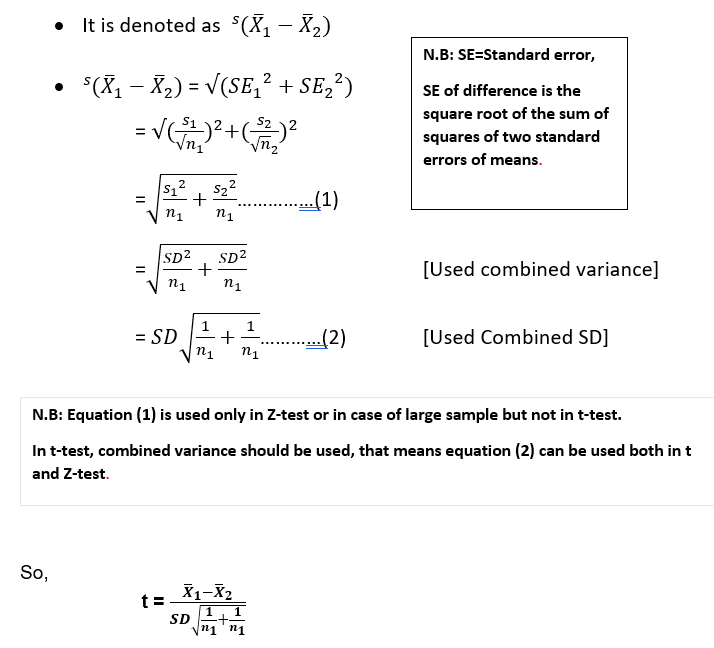
- SE (Standard error) refers to SD (standard deviation) of the distribution of sample.
- It is the approximate SD of a statistical sample population.
- In other word, In statistics, a sample mean deviates from the actual mean of a population,this deviation is the standard error of the mean.
-
Formula to estimate SE
Steps for student’s t-test
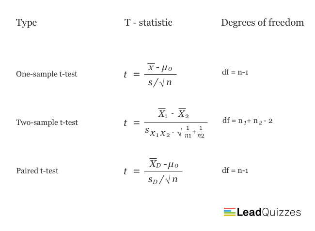
Step 1: Calculate the t-value
Discussed earlier.
Step 2: Calculate the degrees of freedom
Step 3: Determine the critical value
- The critical value represents the predicted or claimed value from which difference between the two values should be considered statistically significant.
- We can find the critical value from the t distribution table below using the degrees of freedom.
N.B: If there’s no specified alpha level, we should use P0.05 (95% confidence level) and we must take the value of two tails.
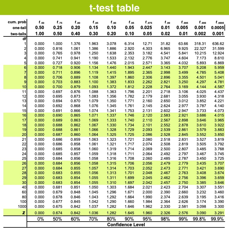
- The column header are the t distribution probabilities (alpha). The row names are the degrees of freedom (df). Student t table gives the probability that the absolute t value with a given degrees of freedom lies above the tabulated value.
Step 4: Compare the t-statistic value to critical value
- If the hypothesis value is equal or less than the critical value at the probability of 5% level, then the result is non significant, that means there have no significant different between two value.
- If non-significant, it can be claim that the null hypothesis (Ho) would be accepted.
- On the other hand, if the result value is greater than the critical value, then there exists a significant difference between them.
So, the null hypothesis would be rejected and an alternative hypothesis should be taken. In this case, the estimates falls in the area of rejection.
Application and examples of t-test
Unpaired Samples
- Two large samples t test (Generally, mean and SD value are known here):
Example
Index of data of 40 boys and 46 girls gave following values.
| Gender | Mean | SD2 |
| Boys | 53.11 | 228.57 |
| Girls | 48.63 | 395.85 |
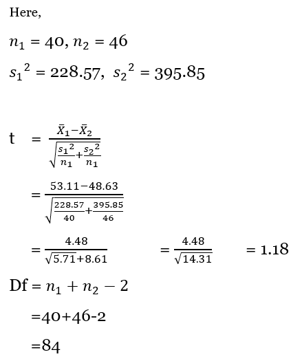
From t table, we can find that the critical t value at 95% confidence level is 1.98 which is greater than our hypothesis value, hence the difference is probably due to chance that means not significant and also the null hypothesis is accepted.
2. Two small samples t test:
- Applied to unpaired data of independent observations made on individuals of two different or separate groups or samples.
- Use only combined variance.
Example
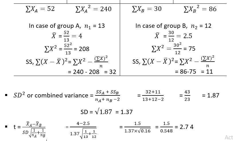
- In a nutritional study, 13 children were given a usual diet plus vitamins A&D tablets while the second comparable group of 12 children was taking the usual diet. After 12 months, the gain is in weight in pounds was noted as given in the table below.
Can we say that vitamins A and D were responsible for this difference?
| Group A | Group B | ||
| XA | XA2 | XB | XB2 |
| 5
3 4 3 2 6 3 2 3 6 7 5 3 |
25
9 16 9 4 36 9 4 9 36 49 25 9 |
1
3 2 4 2 1 3 4 3 2 2 3
|
1
9 4 16 4 1 9 16 9 4 4 9
|
Comments
df = 23
At 23 df the highest obtainable value of ‘t’ at 5% level of significance is 2.069 as found on reference to ‘t’ table. The ‘t’ value in this experiment is found at 2.74 which is much higher than the critical value. The significance is real and null hypothesis rejected.
Paired samples
- It is at applied to paired data of independent observations .
- When each individual give a pair of observations.
- To compare the results of two different lab techniques.
- To study the comparative accuracy of two instruments.
- To study the effect of two drugs.
- To study the role of a factor or cause when the observations are made before and after it’s application.

Example
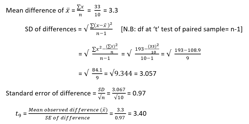
Plant height in cm is given below:
| Serial no. | Height after exposed to light (cm) | Height after exposed to dark (cm) | Difference (cm) |
Differencesquare |
| X1 | X2 | x = X1 – X2 | x2 | |
| 1. | 142 | 138 | 4 | 16 |
| 2. | 140 | 136 | 4 | 16 |
| 3. | 144 | 147 | -3 | 9 |
| 4. | 144 | 139 | 5 | 25 |
| 5. | 142 | 143 | -1 | 1 |
| 6. | 146 | 141 | 5 | 25 |
| 7. | 149 | 143 | 6 | 36 |
| 8. | 150 | 145 | 5 | 25 |
| 9. | 142 | 136 | 6 | 36 |
| 10. | 148 | 146 | 2 | 4 |
| Σ x = 33 | Σ x2 = 193 |
Comment
- df = 9,
- At 5% significant level, ‘t’ value is 2.26.
- Calculated value is so much higher than critical value.
- Significant difference is observed.
- Null hypothesis (Ho) is rejected.
Reference
- Lecture from student’s t-test and comparison of two means by Professor Rakha Hari Sarker.
- Book – Methods in Biostatistics for Medical Students and research workers BK Mahajan.
- Wikipedia.org
Revised by
 Plantlet The Blogging Platform of Department of Botany, University of Dhaka
